水素原子におけるシュレーディンガー方程式の解

本項、水素原子におけるシュレーディンガー方程式の解（すいそげんしにおけるシュレーディンガーほうていしきのかい）では、ハミルトニアンが

${\displaystyle {\hat {H}}=-{\hbar ^{2} \over 2m_{0}}\Delta _{0}-{\hbar ^{2} \over 2m_{1}}\Delta _{1}-{Q \over |{\boldsymbol {x}}_{0}-{\boldsymbol {x}}_{1}|}}$

と書ける二粒子系の時間非依存なシュレーディンガー方程式の厳密解を解く（式中の記号の意味は後述）。

物理学的にはこれは、

• 質量m₀の正の電荷をもつ粒子と質量がm₁負の電荷を持つ粒子がクーロン力により結合している状況において
• 外力は働いておらず、
• 相対論的効果を考えない量子力学の範囲内で、
• 時間に依存しない定常状態の

粒子の波動関数を決定する事を意味する。正の電荷をもつ粒子と負の電荷がそれぞれ陽子と電子だとすればこの系は水素原子に相当するが、一般の価数の原子核を持つ1電子系多価イオン（水素様原子）の系も同一の方程式から解を導ける。この方程式は様々な教科書で取り上げられている^[1][2][3]。

なお、微細構造、超微細構造、ラムシフトなどの効果は、いずれも相対論的な量子力学を必要とする為、本項の対象外である。

シュレーディンガー方程式

本項の目的は、時間非依存なシュレディンガー方程式

${\displaystyle {\hat {H}}\psi ({\boldsymbol {x}}_{0},{\boldsymbol {x}}_{1})=E\psi ({\boldsymbol {x}}_{0},{\boldsymbol {x}}_{1})}$　　…(X1)

でハミルトニアンが

${\displaystyle {\hat {H}}=-{\hbar ^{2} \over 2m_{0}}\Delta _{0}-{\hbar ^{2} \over 2m_{1}}\Delta _{1}-{Q \over |{\boldsymbol {x}}_{0}-{\boldsymbol {x}}_{1}|}}$ …(X2)

と書ける場合の厳密解を求める事である。ここで

ここで

${\displaystyle {\boldsymbol {x}}_{0}=(x_{0},y_{0},z_{0})}$

${\displaystyle {\boldsymbol {x}}_{1}=(x_{1},y_{1},z_{1})}$

はR³の元であり、m₀、m₁、Qは正の定数であり、

${\displaystyle \Delta _{j}={\partial ^{2} \over \partial x_{j}{}^{2}}+{\partial ^{2} \over \partial y_{j}{}^{2}}+{\partial ^{2} \over \partial z_{j}{}^{2}}}$、

であり、ℏは換算プランク定数である。

前述した物理的状況においては、２つの粒子の電荷をそれぞれe₁, −e₂とし、真空の誘電率をε₀とすれば、

${\displaystyle Q={e_{1}e_{2} \over 4\pi \varepsilon _{0}}}$

であるが、本項では一般の正の定数Qに対して解を導くので、必ずしもQが上述の形である事を仮定しない。

重心系への還元

(X1)、(X2)により定義される方程式は、重心系に書き直す事により、より簡単な式に還元できる。２つの粒子の重心

${\displaystyle {\boldsymbol {c}}={m_{0}{\boldsymbol {x}}_{0}+m_{1}{\boldsymbol {x}}_{1} \over m_{0}+m_{1}}}$

と２つの粒子の位置の差

${\displaystyle {\boldsymbol {x}}={\boldsymbol {x}}_{1}-{\boldsymbol {x}}_{0}}$

と換算質量

${\displaystyle \mu ={\frac {m_{0}m_{1}}{m_{0}+m_{1}}}}$

を使うと、ハミルトニアン(X2)は

${\displaystyle {\hat {H}}=-{\hbar ^{2} \over 2(m_{0}+m_{1})}\Delta _{\boldsymbol {c}}-{\hbar ^{2} \over 2\mu }\Delta _{\boldsymbol {x}}-{Q \over |{\boldsymbol {x}}|}}$

と書ける^H13(p416)。

このハミルトニアンは

${\displaystyle {\hat {H}}_{c}=-{\hbar ^{2} \over 2(m_{0}+m_{1})}\Delta _{\boldsymbol {c}}}$　　…(Y1)

${\displaystyle {\hat {H}}_{\boldsymbol {x}}=-{\hbar ^{2} \over 2\mu }\Delta _{\boldsymbol {x}}-{Q \over |{\boldsymbol {x}}|}}$　　…(Y2)

の和である。

(Y1)のハミルトニアンはよく知られた自由粒子のハミルトニアンであり、その連続スペクトルは

${\displaystyle \sigma _{c}({\hat {H}}_{c})=[0,\infty )}$

であり、点スペクトルは

${\displaystyle \sigma _{c}({\hat {H}}_{c})=\emptyset }$

である^H13(p235)。したがって後は非自明な部分である(Y2)のスペクトルを求めれば良いことになる^新井(p263)。そこで以下(Y2)のみ焦点を当てる。

無次元化

適切な値a₀と定数E_aを選び、長さとエネルギーをそれぞれa₀、E_aが1となるように座標変換

${\displaystyle (x',y',z')=(x/a_{0},y/a_{0},z/a_{0})}$

${\displaystyle E'=E/E_{a}}$

してやると、(Y2)のハミルトニアンに関する時間非依存なシュレディンガー方程式は

${\displaystyle -{1 \over 2}\Delta _{{\boldsymbol {x}}'}\psi -{\psi \over |{\boldsymbol {x}}'|}=E'\psi }$　　…(A1)

と無次元化される^{SO96:2.1.1節}

簡単な計算によりa₀、E_aの具体的な値は

${\displaystyle a_{0}={\hbar ^{2} \over \mu Q}}$、${\displaystyle E_{a}={\mu Q^{2} \over \hbar ^{2}}}$　　…(A2)

である事が分かる。

ボーア半径・ハートリー

特に、陽子の質量m₀が電子の質量m₁より遥かに重いと仮定した場合の水素原子の系におけるa₀、E_aは

${\displaystyle Q={e^{2} \over 4\pi \varepsilon _{0}}}$

${\displaystyle \mu =m_{1}\left(1+{m_{1} \over m_{0}}\right)\approx m_{1}}$

より、

${\displaystyle a_{0}={4\pi \varepsilon _{0}\hbar ^{2} \over m_{1}e^{2}}}$、${\displaystyle E_{a}={m_{1}e^{4} \over 16\pi ^{2}\varepsilon _{0}^{2}\hbar ^{4}}}$

である。ここでeは電気素量である。この場合のa₀をボーア半径といい、E_aを基準としたエネルギーの単位をハートリーという^{SO96:2.1.1節}。

求解

本節では(Y2)のハミルトニアンを無次元した

${\displaystyle {\hat {H}}_{{\boldsymbol {x}}'}=-{\hbar ^{2} \over 2\mu }\Delta _{{\boldsymbol {x}}'}-{Q \over |{\boldsymbol {x}}'|}}$ …（A1、再掲）

のスペクトルを求める。なお、本節ではまず変数分離解を求めるが、後述するように実はこのハミルトニアンは変数分離解しか持たない。

求解の方針

(A1)を解く基本的アイデアは、無次元化した座標系(x′,y′,z′) = (x/a₀, y/a₀, z/a₀)を球面座標(r′,θ,φ)に変換するというものだが、直接球面座標を用いると、計算が複雑になる。そこで計算を楽にするため、以下の事実に着目する。

(A1)のハミルトニアンは球対称なポテンシャルを持っており、しかもラプラシアンは回転不変である事が知られているので、(A1)のハミルトニアンは回転不変である。よって(A1)のハミルトニアンは軌道角運動量演算子${\displaystyle ({\hat {L}}_{x},{\hat {L}}_{y},{\hat {L}}_{z})}$と可換である：

${\displaystyle [{\hat {H}}_{{\boldsymbol {x}}'},{\hat {L}}_{x}]=[{\hat {H}}_{{\boldsymbol {x}}'},{\hat {L}}_{y}]=[{\hat {H}}_{{\boldsymbol {x}}'},{\hat {L}}_{z}]=0}$

よって特に、軌道角運動量演算子の自乗ˆL²とも可換である：

${\displaystyle [{\hat {H}}_{{\boldsymbol {x}}'},{\hat {{\boldsymbol {L}}^{2}}}]=0}$

よってˆH_x′はˆL²と同時対角化できるはずである^{[注 1]}、さらに

${\displaystyle [{\hat {{\boldsymbol {L}}^{2}}},{\hat {L}}_{z}]=0}$

である事から、ˆH_x′, ˆL², ˆL_zの３つを同時対角化できるはずである^{[注 1]}。

そこでまず、ˆL², ˆL_zの同時固有関数を求め、これを利用してˆH_x′の固有関数を求める。

ˆL²とˆL_zの同時固有関数

ˆL²とˆL_zの同時固有関数の求め方は「軌道角運動量」の項目に書いてあるので、結論だけを言えば、ℓ = 0, 1, 2, …, m = 0, ±1, ±2, … ±ℓに対し、

${\displaystyle {\hat {{\boldsymbol {L}}^{2}}}\psi =\hbar ^{2}\ell (\ell +1)\psi }$

${\displaystyle {\hat {L}}_{z}\psi =m\hbar \psi }$

を満たす固有関数ψが存在し、ψは極座標で

${\displaystyle \psi (r',\theta ,\varphi )=R(r')P_{\ell }^{|m|}(\cos \theta )\,e^{im\phi }}$ 　　×(規格化定数)　…(B1)

という形で書ける。ここでR(r')は任意の自乗可積分関数であり、P_ℓ^m(z)はルジャンドルの陪多項式

${\displaystyle P_{\ell }{}^{m}(z)={1 \over 2^{\ell }\ell !}(1-z^{2})^{m \over 2}{\operatorname {d} ^{m+\ell } \over \operatorname {d} z^{m+\ell }}(z^{2}-1)^{\ell }}$

である^新井(p277)。

R(r′)の決定

後はR(r′)を決定するだけである。R(r′)を決定するには(B1)を(Y2)のハミルトニアンに入れてシュレディンガー方程式(Y1)を解けば良い。（A1）を式変形すると、

${\displaystyle \left({1 \over 2}\Delta _{{\boldsymbol {x}}'}+{1 \over |{\boldsymbol {x}}'|}+E'\right)\psi =0}$　　 …(W1)

である。ラプラシアンを球面座標(r′,θ,φ)で書き表し、動径方向と球面方向にわけると、

${\displaystyle \Delta _{{\boldsymbol {x}}'}={1 \over r'^{2}}(\Delta _{r'}+\Delta _{S})}$　 …(W2)

と書ける^{武藤11-15(p13)}。ここで

${\displaystyle \Delta _{r'}={\frac {\partial }{\partial r'}}\left(r'^{2}{\frac {\partial }{\partial r'}}\right)}$ 、${\displaystyle \Delta _{S}=-{1 \over \hbar ^{2}}{\hat {{\boldsymbol {L}}^{2}}}}$　　　…(W3)

であり^{武藤11-15(p13)}、ˆL²は軌道角運動量演算子の自乗である。(W1)のラプラシアンを極座標表示した上で(W1)に(B1)の波動関数を代入すると、(B1)がˆL²/ℏ²の固有値ℓ(ℓ+1)に対応する固有関数であった事から、

${\displaystyle {1 \over 2r'^{2}}\left(\Delta _{r'}-\ell (\ell +1)+2r+2r^{2}E'\right)R(r')P_{\ell }^{|m|}(\cos \theta )\,e^{im\phi }=0}$　

すなわち

${\displaystyle \left(\Delta _{r'}-\ell (\ell +1)+2r'+2r'^{2}E'\right)R(r)=0}$　

束縛状態ではEは負の値しか取らないので、記号を簡単にするため

${\displaystyle n:={1 \over {\sqrt {-2E'}}},\rho :={2r' \over n}}$　　　…(W4)

と定義し^{原94(p103-105)}、Rをρの関数とみなすと、

${\displaystyle \rho ^{2}{\frac {\operatorname {d} ^{2}R}{\operatorname {d} \rho ^{2}}}+2\rho {\frac {\operatorname {d} R}{\operatorname {d} \rho }}-\left\{{\frac {\rho ^{2}}{4}}-n\rho +\ell (\ell +1)\right\}R=0}$　…(W5)

が成立する^{石川15(p154)}。

この方程式を解くのは複雑な計算を必要とするので後の章にまわし、ここでは結論のみを述べる。

(W5)の方程式を解くことで各n = 0, 1, 2, …に対し、（(A2)のE_aを単位とした）エネルギー

${\displaystyle E'_{n}=-{\frac {1}{2n^{2}}}}$ ...(B2)

に対する解が見つかる^{新井(p285-286)}。E'_nに対応する固有関数は、

${\displaystyle {\begin{cases}0\leq \ell \leq n-1\\|m|\leq \ell \end{cases}}}$　　　　　　　　　　　　　　　　　　　　　…(B3)

に対してのみ存在し、そのときのR(r)はラゲールの陪関数

${\displaystyle R_{n,\ell }(\rho )=\exp \left(-\rho \right)\rho ^{\ell }L_{n+\ell }^{2\ell +1}\left(2\rho \right)}$　　　　　×規格化定数　　　　　…(B4)

に一致する。ここで

${\displaystyle \rho ={r' \over n}}$、

${\displaystyle L_{k}^{m}(\rho )={\frac {\operatorname {d} ^{m}}{\operatorname {d} \rho ^{m}}}e^{\rho }{\frac {\operatorname {d} ^{k}}{\operatorname {d} \rho ^{k}}}(e^{-\rho }\rho ^{k})}$

である。

規格化定数

3次元空間における体積要素dV = dx′dy′dz′は動径方向の線素dr′と球面方向の面素dS = sinθdθdφを用いて

${\displaystyle \operatorname {d} V=r'^{2}\operatorname {d} r'\operatorname {d} S}$

と書けるので、(B1)におけるψのノルム

${\displaystyle \|\psi \|{}:={\sqrt {\int _{0}^{\pi }|\psi (x',y',z')|^{2}\operatorname {d} V}}}$　　　

も

${\displaystyle \|\psi \|{}:=\|R\|_{r}\|Y\|_{S}}$　　 　…(M1)

と「変数分離」する。ここで

${\displaystyle Y(\theta ,\varphi )=P_{\ell }^{|m|}(\cos \theta )\,e^{im\phi }}$　　

であり、

${\displaystyle \|Y\|_{S}{}:={\sqrt {\int _{0}^{\pi }|Y(\theta ,\phi )|^{2}\operatorname {d} S}}}$　　　　…(M2)

${\displaystyle \|R\|_{r}{}:={\sqrt {\int _{0}^{\infty }|R(r)|^{2}r^{2}\operatorname {d} r}}}$　　　　…(M3)

(M2)のノルムを1にする規格化定数の値は「軌道角運動量」の項目に書いてあり、

${\displaystyle (-1)^{(m+|m|)/2}{\sqrt {{\frac {2\ell +1}{4\pi }}{\frac {(\ell -|m|)!}{(\ell +|m|)!}}\,}}}$

である^原94(p97)。

(M3)のノルムを1にする規格化定数の値の計算は後述するが、結論から言えば規格化定数は

${\displaystyle \left({2 \over n}\right)^{3/2}{\sqrt {\frac {(n-\ell -1)!}{2n(n+\ell )!}}}}$　　　　　...(M5)

である。

結論

無次元化した(A1)をベースにしたこれまでの議論を通常の単位系に戻すことで以下の結論が得られる。

${\displaystyle a_{0}={\hbar ^{2} \over \mu Q}}$

とし、n>0を自然数、ℓ, mを以下を満たす整数とする：

${\displaystyle {\begin{cases}0\leq \ell \leq n-1\\|m|\leq \ell \end{cases}}}$　　　　　　　　　　…('B3'、再掲)　　　　　

このとき(Y2)のハミルトニアンはエネルギー

${\displaystyle E_{n}=-{\frac {\mu Q^{2}}{2\hbar ^{2}n^{2}}}}$

に対し、

${\displaystyle {\hat {{\boldsymbol {L}}^{2}}}\psi =\hbar ^{2}\ell (\ell +1)\psi }$

${\displaystyle {\hat {L}}_{z}\psi =m\hbar \psi }$

を満たす固有関数

${\displaystyle \psi _{n,\ell ,m}(r,\theta ,\phi )=R_{n,\ell }(r)Y_{lm}(\theta ,\phi )=\exp(-\rho _{n})\rho _{n}{}^{\ell }L_{n+\ell }^{2\ell +1}(2\rho _{n})P_{\ell }^{|m|}(\cos \theta )\,e^{im\phi }}$ 　×(規格化定数)　　…(B5)

を持つ。ここで

${\displaystyle P_{\ell }{}^{m}(z)={1 \over 2^{\ell }\ell !}(1-z^{2})^{m \over 2}{\operatorname {d} ^{m+\ell } \over \operatorname {d} z^{m+\ell }}(z^{2}-1)^{\ell }}$、

${\displaystyle L_{k}^{m}(\rho )={\frac {\operatorname {d} ^{m}}{\operatorname {d} \rho ^{m}}}e^{\rho }{\frac {\operatorname {d} ^{k}}{\operatorname {d} \rho ^{k}}}(e^{-\rho }\rho ^{k})}$

${\displaystyle \rho _{n}={r \over na_{0}}}$

であり、規格化定数は

${\displaystyle (-1)^{(m+|m|)/2}{\sqrt {\left({2 \over na_{0}}\right)^{3}{\frac {2\ell +1}{4\pi }}{\frac {(\ell -|m|)!}{(\ell +|m|)!}}{\frac {(n-\ell -1)!}{2n(n+\ell )!}}}}}$

である。

以上では変数分離により発見的に解を求めたため、(B3)、(B5)に書いたものが解である事は間違いないものの、それ以外に解があるかどうかは不明である。しかし実はこれ以外に解がない事が知られている^{H13(p399-400)}。

連続スペクトルに相当する部分は、物理的にいえば水素原子がイオン化している状態であり、したがって電子が陽子から逃れていってしまっている^H13(p399)。なお、固有関数の和

${\displaystyle \sum _{n,\ell ,m}a_{n,\ell ,m}\psi _{n,\ell ,m}(r,\theta ,\phi )}$ s.t. ${\displaystyle \sum _{n,\ell ,m}a_{n,\ell ,m}{}^{2}<\infty }$

の形に書けるのは、ˆH_xの負のスペクトルに対応するベクトルだけで、正のスペクトルに対応するベクトルはこの方法では表記できない^H13(p399)。

量子数

ハミルトニアン(Y2)の固有関数(B5)に登場する２つの変数は以下のように呼ばれる：

• nは主量子数と呼ばれ、ˆH_xのエネルギー固有値の大きさを司っている。
• ℓは軌道角運動量量子数（方位量子数）と呼ばれ、ˆL²の固有値の大きさを司っている。
• mは磁気量子数（軌道磁気量子数）と呼ばれ、ˆL_zの固有値の大きさを司っている。

なお、n−ℓ−1は、動径方向の波動関数の節の数を表している^[要出典]。

化学的意味

3つの量子数のうち、n, ℓには以下のような化学的意味がある：

• 主量子数 n は電子殻の K殻、L殻、M殻、…に対応している。
• 方位量子数 ℓ はs軌道、p軌道、d軌道、f軌道、g軌道…に対応している。

水素原子において、s軌道, p軌道, d軌道, f軌道…のエネルギー準位は縮退している。これはエネルギー固有値が、E = −E_h / 2n²となり、ℓやmに依存しないためである。なお、水素原子に磁場をかけると、これらのエネルギー準位は、スピン部分を無視して考えた場合、磁気量子数mの違いにより分裂する(→ゼーマン効果)。電場をかけた場合も、シュタルク効果によって分裂する。このとき、異なるℓの軌道同士の線形結合をとった混成軌道がハミルトニアンの固有状態となる。

リュードベリ定数

エネルギー準位がE_nにある電子がエネルギー準位がE_n′に落ちると、

${\displaystyle E_{n}-E_{n'}={\frac {\mu Q^{2}}{2\hbar ^{2}}}\left({1 \over n'^{2}}-{1 \over n^{2}}\right)}$

のエネルギーが

${\displaystyle E_{n}-E_{n'}={\hbar c \over \lambda }}$

を満たす波長λの光となって放出される。したがって

${\displaystyle {1 \over \lambda }={\frac {\mu Q^{2}}{2\hbar ^{3}c}}\left({1 \over n'^{2}}-{1 \over n^{2}}\right)}$

水素原子の場合、すなわち

${\displaystyle Q={e^{2} \over 4\pi \varepsilon _{0}}}$

の場合の上式右辺の定数、もしくはその定数に対して近似

${\displaystyle \mu =m_{1}\left(1+{m_{1} \over m_{0}}\right)\approx m_{1}}$

を行ったときの値をリュードベリ定数という。

(W5)の解

本節の目的は、微分方程式(W5)を解き、(B3)、(B4)を導出することである。

ラゲールの陪方程式にあてはめる

本節では式(W5)をさらに式変形することで、(W5)をラゲールの陪方程式（詳細後述）で書き表せる事を示す。ラゲールの陪方程式の解は特殊関数で書けることが知られているので、これにより式(W5)が解けることになる。この目標に達するため、以下の3ステップを踏む。

• ρが十分小さいという条件下(W5)の近似解を求める。
• ρが十分大きいという条件下(W5)の近似解を求める。
• 上記2ステップの結論を参考にして、(W5)の厳密解を変数変換し、(W5)をラゲールの陪方程式に（近似なしで）変形する。

ρが十分小さい場合の(W5)の近似解

(W5)におけるRの係数はρが十分小さいところではℓ(ℓ+1)と近似できるので、(W5)は

${\displaystyle \rho ^{2}{\frac {\operatorname {d} ^{2}R}{\operatorname {d} \rho ^{2}}}+2\rho {\frac {\operatorname {d} R}{\operatorname {d} \rho }}-\ell (\ell +1)R=0}$

と近似できる^{石川15(p155)}。

この形の方程式はオイラーの微分方程式の解法に準ずる方法で解ける。その解は

の形で書ける。

ρが十分大きい場合の(W5)の近似解

(W5)式をρ²で割った上でρ → ∞の極限をとることで、ρが十分大きいところでは(W5)は

となる事がわかる。簡単な計算から上記の方程式の一般解は

${\displaystyle R(\rho )=\mathrm {e} ^{\rho \over 2}}$、${\displaystyle \mathrm {e} ^{-\rho \over 2}}$

もしくはこれらの線形和である。e^ρ/2は発散する不適切な解となるので、

である。

(W5)からのラゲールの陪多項式の導出

(C1)、(C2)を参考に、(W5)の厳密解R(ρ)を

の形に変数変換する。一般に3つの関数の積の微分は公式

${\displaystyle {\begin{aligned}(fgh)'&=f'gh+fg^{'}h+fgh'\\(fgh)''&=(f''gh+fg''h+fgh'')+2(f'g'h+fg'h'+f'gh')\end{aligned}}}$

を満たすので、(W5)の第一項、および第二項は、

${\displaystyle {\begin{array}{lccl}\displaystyle \rho ^{2}{\frac {\operatorname {d} ^{2}R}{\operatorname {d} \rho ^{2}}}&=&{\frac {\operatorname {d} }{\operatorname {d} \rho }}\left\{\rho ^{\ell }u(\rho )\mathrm {e} ^{-{\frac {\rho }{2}}}\right\}&=&\ell \rho ^{\ell -1}u(\rho )\mathrm {e} ^{-{\frac {\rho }{2}}}+\rho ^{\ell }\rho '\mathrm {e} ^{-{\frac {\rho }{2}}}-{\frac {1}{2}}\rho ^{\ell }u(\rho )\mathrm {e} ^{-{\frac {\rho }{2}}}\\\displaystyle \rho {\frac {\operatorname {d} R}{\operatorname {d} \rho }}&=&{\frac {\operatorname {d} ^{2}}{\operatorname {d} \rho ^{2}}}\left\{\rho ^{\ell }u(\rho )\mathrm {e} ^{-{\frac {\rho }{2}}}\right\}&=&\displaystyle \ell (\ell -1)\rho ^{\ell -2}u(\rho )\mathrm {e} ^{-{\frac {\rho }{2}}}+\rho ^{\ell }\rho ''\mathrm {e} ^{-{\frac {\rho }{2}}}+{\frac {1}{4}}\rho ^{\ell }u(\rho )\mathrm {e} ^{-{\frac {\rho }{2}}}\\&&&+&\displaystyle 2\left\{\ell \rho ^{\ell -1}\rho '\mathrm {e} ^{-{\frac {\rho }{2}}}-{\frac {1}{2}}\rho ^{\ell }\rho '\mathrm {e} ^{-{\frac {\rho }{2}}}-{\frac {1}{2}}\ell \rho ^{\ell -1}u(\rho )\mathrm {e} ^{-{\frac {\rho }{2}}}\right\}\end{array}}}$　　

である。上式を(W5)に代入すると、すべての項にe^−ρ/2が掛かっていることがわかる。よって各項をe^−ρ/2で割った上で式を整理して、

を得る。この式の両辺をρ^ℓ−1で割ると、

となる^{石川15(p155)}。こうして得た式(6.12)は下記の式(6.13)に示したラゲールの陪方程式（ラゲール陪関数）の形になっている。

${\displaystyle \rho {\frac {\operatorname {d} ^{2}u(\rho )}{\operatorname {d} \rho ^{2}}}+(m+1-\rho ){\frac {\operatorname {d} u(\rho )}{\operatorname {d} \rho }}+(k-m)u(\rho )=0}$ …(C4)

ラゲールの陪方程式の解u(ρ)はラゲールの陪多項式（ラゲール陪関数）と呼ばれる形の定数倍になることが知られている。ラゲールの陪多項式（ラゲール陪関数）Lm
k(ρ)は下記のように定義される。

${\displaystyle L_{k}^{m}(\rho )={\frac {\operatorname {d} ^{m}}{\operatorname {d} \rho ^{m}}}e^{\rho }{\frac {\operatorname {d} ^{k}}{\operatorname {d} \rho ^{k}}}(e^{-\rho }\rho ^{k})\quad \rho ={2r \over n}}$

ここで、kは

${\displaystyle 0\leq k\leq m}$ …(C5)

を満たす整数である。

よって(C4)の解は

${\displaystyle u(\rho )=L_{n+\ell }^{2\ell +1}(\rho )}$ ×(規格化定数)

となる。これを変数変換の式(C3)に代入して

${\displaystyle R(\rho )=\rho ^{\ell }L_{n+\ell }^{2\ell +1}(\rho )\exp \left(-{\frac {\rho }{2}}\right)}$ ×(規格化定数) …(C6)

を得る。

ラゲール陪多項式の係数の条件式(C4)から、${\displaystyle hoge\ell }$は

${\displaystyle 0\leq \ell \leq n-1}$ …(C7)

を満たす整数でなければならない。

規格化定数(M5)の導出

規格化定数をC′とすると、規格化条件

${\displaystyle \int _{0}^{\infty }|R(r')|^{2}r'^{2}\operatorname {d} r'=1}$

は、(W2)、(W4)より、

${\displaystyle {\begin{array}{lcl}\displaystyle 1=\int _{0}^{\infty }|R(r')|^{2}r'^{2}\operatorname {d} r&=&\displaystyle {n^{3} \over 8}\int _{0}^{\infty }R(\rho )^{2}\rho ^{2}\operatorname {d} \rho \\&=&\displaystyle {n^{3}C' \over 8}\int _{0}^{\infty }\rho ^{2\ell +2}\{L_{n+\ell }^{2\ell +1}(\rho )\}^{2}\exp \left(-\rho \right)\operatorname {d} \rho \\\\\end{array}}}$ …(D1)

ラゲールの陪多項式（ラゲール陪関数）は下記の直交性を満たすことが知られている

${\displaystyle {\begin{aligned}\int _{0}^{\infty }z^{m}\exp(-z)L_{k}^{m}(z)L_{\ell }^{m}(z)\operatorname {d} z&={\frac {(k!)^{3}}{(k-m)!}}\delta _{k\ell }\\\int _{0}^{\infty }z^{m+1}\exp(-z)\{L_{k}^{m}(z)\}^{2}\operatorname {d} z&=(2k+1-m){\frac {(k!)^{3}}{(k-m)!}}\end{aligned}}}$

ので、後者の式を(D1)に対して用いる事で、

${\displaystyle \displaystyle \int _{0}^{\infty }\rho ^{2\ell +2}\{L_{n+\ell }^{2\ell +1}(\rho )\}^{2}\exp \left(-\rho \right)\operatorname {d} \rho =\displaystyle (2n){\frac {[(n+\ell )!]^{3}}{(n-\ell -1)!}}}$

これが(D1)の左辺である1と等しいことから、規格化定数C′について解く事で

${\displaystyle C'=\left({2 \over n}\right)^{3/2}{\sqrt {\frac {(n-\ell -1)!}{2n[(n+\ell )!]^{3}}}}}$　　…(D2)

が得られる。

なお、無次元化する前のハミルトニアン(Y2)に対する規格化定数は、変数変換

${\displaystyle \int _{0}^{\infty }|R(r)|^{2}r^{2}\operatorname {d} r={1 \over a_{0}}^{3}\int _{0}^{\infty }|R(r')|^{2}r'^{2}\operatorname {d} r'}$

の分だけ(D2)のものとはずれるので、(Y2)に対する規格化定数は、

${\displaystyle C=\left({2 \over na_{0}}\right)^{3/2}{\sqrt {\frac {(n-\ell -1)!}{2n[(n+\ell )!]^{3}}}}}$　　…(D3)

となる^原94(p106)。

具体的な値

水素原子の波動関数のℓ = 0~3における角因子は以下のようになる。ここでΘ(θ)、Φ(φ)はそれぞれ、動径方向の関数

${\displaystyle Y(\theta ,\varphi )=P_{\ell }^{|m|}(\cos \theta )\,e^{im\varphi }}$　

の右辺の積の第一成分と第二成分を規格化したものである。なお、Φ(φ)の指数関数の虚数部分はオイラーの公式により一対のΦ(φ)関数の一次結合で書き換えられる。

ℓ	m	Φ(φ)	Θ(θ)		Φ(φ)Θ(θ)（極座標）	Φ(φ)Θ(θ)（直交座標）	記号
0	0	${\displaystyle {\frac {1}{\sqrt {2\pi }}}}$	${\displaystyle {\frac {1}{\sqrt {2}}}}$		${\displaystyle {\frac {1}{2{\sqrt {\pi }}}}}$	${\displaystyle {\frac {1}{2{\sqrt {\pi }}}}}$	${\displaystyle {\mbox{s}}\,}$
1	0	${\displaystyle {\frac {1}{\sqrt {2\pi }}}}$	${\displaystyle {\sqrt {\frac {3}{2}}}\cos \theta }$		${\displaystyle {\frac {1}{2}}{\sqrt {\frac {3}{\pi }}}\cos \theta }$	${\displaystyle {\frac {1}{2}}{\sqrt {\frac {3}{\pi }}}{\frac {z}{r}}}$	${\displaystyle {\mbox{p}}_{z}\,}$
1	+1	${\displaystyle {\frac {1}{\sqrt {2\pi }}}\exp(i\phi )}$	${\displaystyle {\frac {\sqrt {3}}{2}}\sin \theta }$	${\displaystyle {\Bigg \{}}$	${\displaystyle {\frac {1}{2}}{\sqrt {\frac {3}{\pi }}}\sin \theta \cos \phi }$	${\displaystyle {\frac {1}{2}}{\sqrt {\frac {3}{\pi }}}{\frac {x}{r}}}$	${\displaystyle {\mbox{p}}_{x}\,}$
1	-1	${\displaystyle {\frac {1}{\sqrt {2\pi }}}\exp(-i\phi )}$	${\displaystyle {\frac {\sqrt {3}}{2}}\sin \theta }$		${\displaystyle {\frac {1}{2}}{\sqrt {\frac {3}{\pi }}}\sin \theta \sin \phi }$	${\displaystyle {\frac {1}{2}}{\sqrt {\frac {3}{\pi }}}{\frac {y}{r}}}$	${\displaystyle {\mbox{p}}_{y}\,}$
2	0	${\displaystyle {\frac {1}{\sqrt {2\pi }}}}$	${\displaystyle {\frac {1}{2}}{\sqrt {\frac {5}{2}}}(3\cos ^{2}\theta -1)}$		${\displaystyle {\frac {1}{4}}{\sqrt {\frac {5}{\pi }}}(3\cos ^{2}\theta -1)}$	${\displaystyle {\frac {1}{4}}{\sqrt {\frac {5}{\pi }}}{\frac {2z^{2}-x^{2}-y^{2}}{r^{2}}}}$	${\displaystyle {\mbox{d}}_{3z^{2}-r^{2}}}$
2	+1	${\displaystyle {\frac {1}{\sqrt {2\pi }}}\exp(i\phi )}$	${\displaystyle {\frac {\sqrt {15}}{2}}\sin \theta \cos \theta }$	${\displaystyle {\Bigg \{}}$	${\displaystyle {\frac {1}{2}}{\sqrt {\frac {15}{\pi }}}\sin \theta \cos \theta \cos \phi }$	${\displaystyle {\frac {1}{2}}{\sqrt {\frac {15}{\pi }}}{\frac {zx}{r^{2}}}}$	${\displaystyle {\mbox{d}}_{zx}\,}$
2	-1	${\displaystyle {\frac {1}{\sqrt {2\pi }}}\exp(-i\phi )}$	${\displaystyle {\frac {\sqrt {15}}{2}}\sin \theta \cos \theta }$		${\displaystyle {\frac {1}{2}}{\sqrt {\frac {15}{\pi }}}\sin \theta \cos \theta \sin \phi }$	${\displaystyle {\frac {1}{2}}{\sqrt {\frac {15}{\pi }}}{\frac {yz}{r^{2}}}}$	${\displaystyle {\mbox{d}}_{yz}\,}$
2	+2	${\displaystyle {\frac {1}{\sqrt {2\pi }}}\exp(2i\phi )}$	${\displaystyle {\frac {\sqrt {15}}{4}}\sin ^{2}\theta }$	${\displaystyle {\Bigg \{}}$	${\displaystyle {\frac {1}{4}}{\sqrt {\frac {15}{\pi }}}\sin ^{2}\theta \cos 2\phi }$	${\displaystyle {\frac {1}{4}}{\sqrt {\frac {15}{\pi }}}{\frac {x^{2}-y^{2}}{r^{2}}}}$	${\displaystyle {\mbox{d}}_{x^{2}-y^{2}}}$
2	-2	${\displaystyle {\frac {1}{\sqrt {2\pi }}}\exp(-2i\phi )}$	${\displaystyle {\frac {\sqrt {15}}{4}}\sin ^{2}\theta }$		${\displaystyle {\frac {1}{4}}{\sqrt {\frac {15}{\pi }}}\sin ^{2}\theta \sin 2\phi }$	${\displaystyle {\frac {1}{2}}{\sqrt {\frac {15}{\pi }}}{\frac {xy}{r^{2}}}}$	${\displaystyle {\mbox{d}}_{xy}\,}$
3	0	${\displaystyle {\frac {1}{\sqrt {2\pi }}}}$	${\displaystyle {\frac {1}{2}}{\sqrt {\frac {7}{2}}}(5\cos ^{3}\theta -3\cos \theta )}$		${\displaystyle {\frac {1}{4}}{\sqrt {\frac {7}{\pi }}}(5\cos ^{3}\theta -3\cos \theta )}$	${\displaystyle {\frac {1}{4}}{\sqrt {\frac {7}{\pi }}}{\frac {z(2z^{2}-3x^{2}-3y^{2})}{r^{3}}}}$	${\displaystyle {\mbox{f}}_{z(5z^{2}-3r^{2})}}$
3	+1	${\displaystyle {\frac {1}{\sqrt {2\pi }}}\exp(i\phi )}$	${\displaystyle {\frac {1}{4}}{\sqrt {\frac {21}{2}}}(5\cos ^{2}\theta -1)\sin \theta }$	${\displaystyle {\Bigg \{}}$	${\displaystyle {\frac {1}{4}}{\sqrt {\frac {21}{2\pi }}}(5\cos ^{2}\theta -1)\sin \theta \cos \phi }$	${\displaystyle {\frac {1}{4}}{\sqrt {\frac {21}{2\pi }}}{\frac {x(5z^{2}-r^{2})}{r^{3}}}}$	${\displaystyle {\mbox{f}}_{x(5z^{2}-r^{2})}}$
3	-1	${\displaystyle {\frac {1}{\sqrt {2\pi }}}\exp(-i\phi )}$	${\displaystyle {\frac {1}{4}}{\sqrt {\frac {21}{2}}}(5\cos ^{2}\theta -1)\sin \theta }$		${\displaystyle {\frac {1}{4}}{\sqrt {\frac {21}{2\pi }}}(5\cos ^{2}\theta -1)\sin \theta \sin \phi }$	${\displaystyle {\frac {1}{4}}{\sqrt {\frac {21}{2\pi }}}{\frac {y(5z^{2}-r^{2})}{r^{3}}}}$	${\displaystyle {\mbox{f}}_{y(5z^{2}-r^{2})}}$
3	+2	${\displaystyle {\frac {1}{\sqrt {2\pi }}}\exp(2i\phi )}$	${\displaystyle {\frac {\sqrt {105}}{4}}\cos \theta \sin ^{2}\theta }$	${\displaystyle {\Bigg \{}}$	${\displaystyle {\frac {1}{4}}{\sqrt {\frac {105}{\pi }}}\cos \theta \sin ^{2}\theta \cos 2\phi }$	${\displaystyle {\frac {1}{4}}{\sqrt {\frac {105}{\pi }}}{\frac {z(x^{2}-y^{2})}{r^{3}}}}$	${\displaystyle {\mbox{f}}_{z(x^{2}-y^{2})}}$
3	-2	${\displaystyle {\frac {1}{\sqrt {2\pi }}}\exp(-2i\phi )}$	${\displaystyle {\frac {\sqrt {105}}{4}}\cos \theta \sin ^{2}\theta }$		${\displaystyle {\frac {1}{4}}{\sqrt {\frac {105}{\pi }}}\cos \theta \sin ^{2}\theta \sin 2\phi }$	${\displaystyle {\frac {1}{2}}{\sqrt {\frac {105}{\pi }}}{\frac {xyz}{r^{3}}}}$	${\displaystyle {\mbox{f}}_{xyz}\,}$
3	+3	${\displaystyle {\frac {1}{\sqrt {2\pi }}}\exp(3i\phi )}$	${\displaystyle {\frac {1}{4}}{\sqrt {\frac {35}{2}}}\sin ^{3}\theta }$	${\displaystyle {\Bigg \{}}$	${\displaystyle {\frac {1}{4}}{\sqrt {\frac {35}{2\pi }}}\sin ^{3}\theta \cos 3\phi }$	${\displaystyle {\frac {1}{4}}{\sqrt {\frac {35}{2\pi }}}{\frac {x(x^{2}-3y^{2})}{r^{3}}}}$	${\displaystyle {\mbox{f}}_{x(x^{2}-3y^{2})}}$
3	-3	${\displaystyle {\frac {1}{\sqrt {2\pi }}}\exp(-3i\phi )}$	${\displaystyle {\frac {1}{4}}{\sqrt {\frac {35}{2}}}\sin ^{3}\theta }$		${\displaystyle {\frac {1}{4}}{\sqrt {\frac {35}{2\pi }}}\sin ^{3}\theta \sin 3\phi }$	${\displaystyle {\frac {1}{4}}{\sqrt {\frac {35}{2\pi }}}{\frac {y(3x^{2}-y^{2})}{r^{3}}}}$	${\displaystyle {\mbox{f}}_{y(3x^{2}-y^{2})}}$

原子番号Zの水素様原子の動径関数は以下のようになる。

${\displaystyle {\begin{aligned}R_{1\mathrm {s} }&=2\left({\frac {Z}{a_{0}}}\right)^{3/2}\exp \left(-{\frac {Zr}{a_{0}}}\right)\\R_{2\mathrm {s} }&={\frac {1}{2{\sqrt {2}}}}\left({\frac {Z}{a_{0}}}\right)^{3/2}\left(2-{\frac {Zr}{a_{0}}}\right)\exp \left(-{\frac {Zr}{2a_{0}}}\right)\\R_{2\mathrm {p} }&={\frac {1}{2{\sqrt {6}}}}\left({\frac {Z}{a_{0}}}\right)^{3/2}{\frac {Zr}{a_{0}}}\exp \left(-{\frac {Zr}{2a_{0}}}\right)\\R_{3\mathrm {s} }&={\frac {2}{81{\sqrt {3}}}}\left({\frac {Z}{a_{0}}}\right)^{3/2}\left(27-{\frac {18Zr}{a_{0}}}+{\frac {2Z^{2}r^{2}}{a_{0}^{2}}}\right)\exp \left(-{\frac {Zr}{3a_{0}}}\right)\\R_{3\mathrm {p} }&={\frac {4}{81{\sqrt {6}}}}\left({\frac {Z}{a_{0}}}\right)^{3/2}\left(6-{\frac {Zr}{a_{0}}}\right){\frac {Zr}{a_{0}}}\exp \left(-{\frac {Zr}{3a_{0}}}\right)\\R_{3\mathrm {d} }&={\frac {4}{81{\sqrt {30}}}}\left({\frac {Z}{a_{0}}}\right)^{3/2}{\frac {Z^{2}r^{2}}{a_{0}^{2}}}\exp \left(-{\frac {Zr}{3a_{0}}}\right)\\R_{4\mathrm {s} }&={\frac {1}{768}}\left({\frac {Z}{a_{0}}}\right)^{3/2}\left(192-{\frac {144Zr}{a_{0}}}+{\frac {24Z^{2}r^{2}}{a_{0}^{2}}}-{\frac {Z^{3}r^{3}}{a_{0}^{3}}}\right)\exp \left(-{\frac {Zr}{4a_{0}}}\right)\\R_{4\mathrm {p} }&={\frac {1}{256{\sqrt {15}}}}\left({\frac {Z}{a_{0}}}\right)^{3/2}\left(80-{\frac {20Zr}{a_{0}}}+{\frac {Z^{2}r^{2}}{a_{0}^{2}}}\right){\frac {Zr}{a_{0}}}\exp \left(-{\frac {Zr}{4a_{0}}}\right)\\R_{4\mathrm {d} }&={\frac {1}{768{\sqrt {5}}}}\left({\frac {Z}{a_{0}}}\right)^{3/2}\left(12-{\frac {Zr}{a_{0}}}\right){\frac {Z^{2}r^{2}}{a_{0}^{2}}}\exp \left(-{\frac {Zr}{4a_{0}}}\right)\\R_{4\mathrm {f} }&={\frac {1}{768{\sqrt {35}}}}\left({\frac {Z}{a_{0}}}\right)^{3/2}{\frac {Z^{3}r^{3}}{a_{0}^{3}}}\exp \left(-{\frac {Zr}{4a_{0}}}\right)\end{aligned}}}$

1s軌道の動径関数
2s軌道の動径関数	2p軌道の動径関数
3s軌道の動径関数	3p軌道の動径関数	3d軌道の動径関数
4s軌道の動径関数	4p軌道の動径関数	4d軌道の動径関数	4f軌道の動径関数

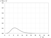
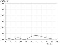
動径関数を2乗しr²を掛けた動径分布r²R(r)²は、核の中心からのある距離における電子の存在確率に相当する。

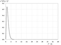1s軌道の動径分布
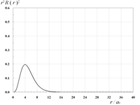2s軌道の動径分布	2p軌道の動径分布
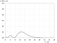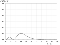3s軌道の動径分布	3p軌道の動径分布	3d軌道の動径分布
4s軌道の動径分布	4p軌道の動径分布	4d軌道の動径分布	4f軌道の動径分布

詳しくは電子配置の項を参照のこと。

脚注

注釈

1. ^ ^{a b} 厳密にいうと、量子力学で扱わねばならない無限次元の線形代数においては、２つの作用素が同時対角化可能であること(強可換性)は一般には交換子が0になる事（可換性）よりも強い条件である^新井(p179)。したがって可換性から同時対角化可能性を結論付けるのは本当は正しい推論ではない。したがってここはあくまで、交換子が0になってるため同時対角化可能で「あろう」という推測の元、発見的解法を試みたと解釈すべきである。

出典

参考文献

• 書籍
  • [新井97] 新井朝雄 (1997/1/25). ヒルベルト空間と量子力学. 共立講座２１正規の数学１６. 共立出版 
  • [原94] 原康夫『５ 量子力学』岩波書店〈岩波基礎物理シリーズ〉、1994年6月6日。ISBN 978-4000079259。 
  • [H13] Brian C.Hall (2013/7/1). Quantum Theory for Mathematicians. Graduate Texts in Mathematics 267. Springer 
  • [SO96] Attila Szabo, Neil S. Ostlund (1996/7/2). Modern Quantum Chemistry: Introduction to Advanced Electronic Structure Theory. Dover Books on Chemistry. Dover Publications. ISBN 978-0486691862 
    • 邦訳：A. ザボ, N.S. オストランド 大野公男, 望月祐志, 阪井健男訳 (1996/7/2). 新しい量子化学―電子構造の理論入門〈上〉、〈下〉. 東京大学出版会 
• レクチャーノート
  • [武藤11-15]武藤一雄. “第１５章 中心力ポテンシャルでの束縛状態” (pdf). 量子力学第二 平成２３年度　学部　５学期 . 東京工業大学. 2017年8月13日閲覧。
  • [石川15] 石川健三 (2015年1月21日). “量子力学” (pdf). 北海道大学理学部. 2017年8月13日閲覧。

関連項目

• シュレーディンガー方程式
• 球面調和関数
• ラゲールの陪多項式
• 水素原子

外部リンク

• 水素原子の電子分布の計算